Clustering algorithms identify groups of samples that are similar with each other.
Consider a population of dogs, where you want to separate the population into dog breeds. You suspect that there are k different breeds of dog, though you don’t know what they are. You take several measurements of the dogs, including height, fluffiness, and darkness. Assume that fluffiness and darkness are ratings between 1 and 100.
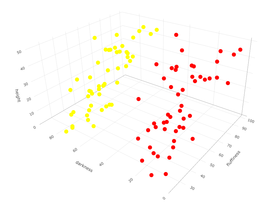
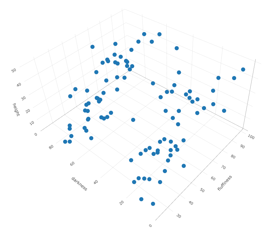
K-means and K-medoids can help you identify k separate groups within your population, by looking at features you provide them, in this case height, fluffiness and roundness of muzzle. Below is some sample data with those 3 measurements.
Using those three features, k-means and k-medoids finds k numbers of groups in the space that are closest to each other.
K-means
K-means will randomly choose k dogs as the center of each cluster. It then assigns the remaining dogs by looking at which cluster center it is closest to in terms of distance. Note there are different distance measures you can use. Then we have all dogs grouped into k clusters. They represent possible breeds 1, 2, 3, … k.
For each cluster, we take the mean value of height, fluffiness and muzzle roundness, create k imaginary dogs with those features, and use those as the new cluster centers. We repeat the previous exercise of assigning all dogs to the nearest cluster center. If the groups are the same as before, we’re done.
Otherwise, we take the mean value again for each cluster to create the imaginary dogs again, assign each real dog to closest imaginary dog, ending up again with k groups of dogs. We keep repeating this until we see no change in groups.
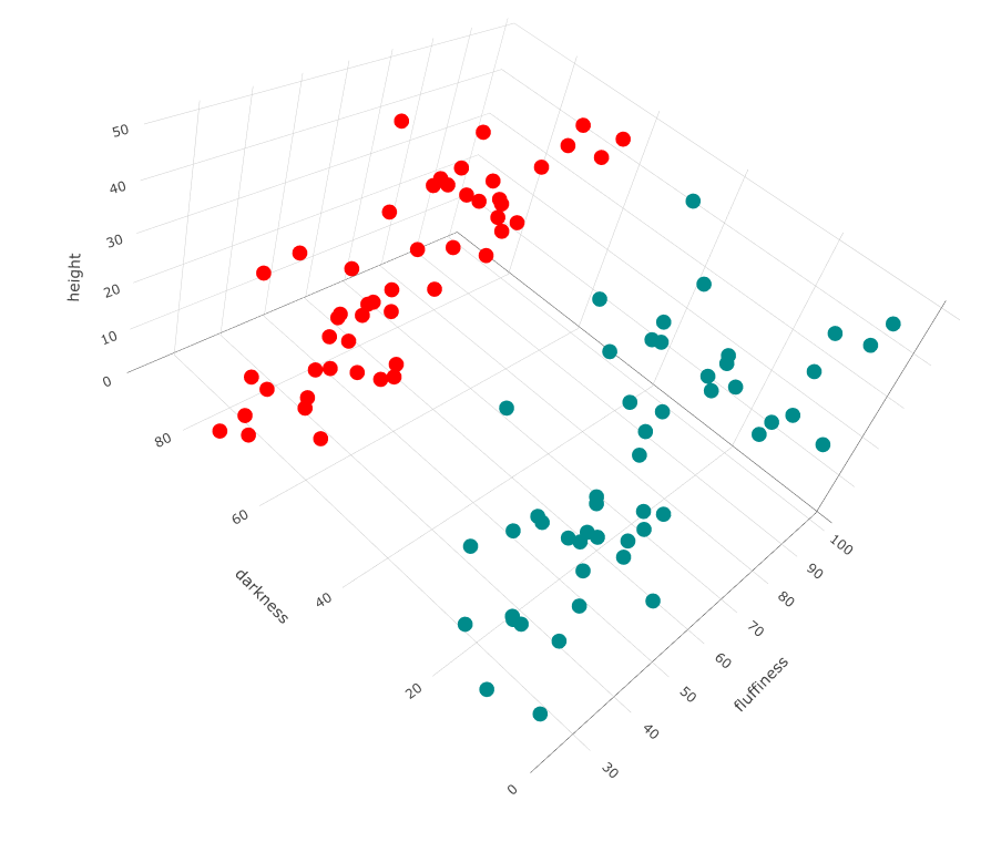
The samples for the previous plot happen to be contained in a data frame in the R language. I’ve called the data frame variable df, with columns called height, fluffiness and darkness. We can run k-means on this in R as follows, first with k = 2 breeds.
# Load the plotting library
library(plotly)

# Run k-means with k = 2 cluster centers
cl <- kmeans(df, centers=2)

# Plot output
plot_ly(df, type="scatter3d", x= ~height, y= ~fluffiness, z= ~darkness,
        # highlight different breeds k-means finds with different colors
        color= as.factor(cl$cluster), colors= c('red','darkcyan'))
Now, run it for 4:
# Run kmeans with 4 centers
cl <- kmeans(df,centers=4)

# Plot
plot_ly(df, type="scatter3d",
        x= ~height, y= ~fluffiness, z= ~darkness,
        color= as.factor(cl$cluster),
        colors= c('red','darkcyan','blue', 'yellow'))
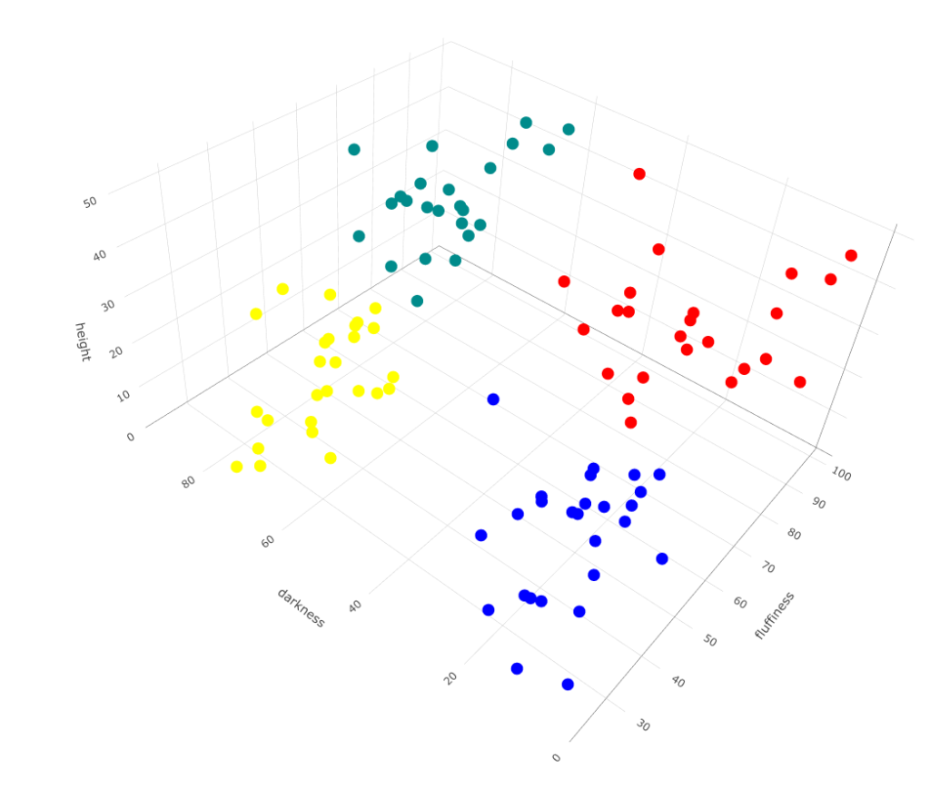
You’ll notice some drawbacks of this k-means. Depending on the initial dog you choose for the cluster center, you may not get the same result in the end.
In summary, the steps are:
Choose k initial cluster centers, and assign samples to clusters which is most similar to the cluster center.
Repeat the following until no change to cluster centers:
- Determine the mean value of the data samples in the cluster, and make these the cluster centers
- Assign data samples to the cluster to which the sample is most similar to the cluster center
| Pros | Cons |
| ✔ Efficient compared to k-medoids | ✘ Sensitive to outliers ✘ Doesn’t guarantee optimal global solution ✘ Results can vary based on initial clusters |
K-medoids
In K-medoids, we start off the same as K-means. We randomly choose k dogs as the cluster centers, and assign the remaining dogs to the closest cluster center dogs.
However rather than averaging the features and making an imaginary dog, we make a calculation called the ‘cost’ of a model, made of summing up the distance between each dog and the cluster center dog that each dog belongs to.
What we want to do is find the clusters that minimize the cost. We do this by going through all the dogs that are not cluster centers, and pretending that dog is the cluster center. We work out again which cluster each dog should belong to, and calculate the new ‘cost’ by summing up distances again. If the total ‘cost’ is lower, then we keep this configuration.
In summary:
Choose k initial cluster centers, and assign samples to cluster to which the sample is most similar to the cluster center (same as k-means).
Calculate the cost of the model by summing up distances between points from their cluster center.
For all points that are not cluster centers (a.k.a non-representative samples):
-
- Take the point as a new possible cluster center
- Reassign samples to the closest center
- Calculate the cost from this new center
- If the cost is lower, make this the new cluster center
| Pros | Cons |
| ✔ Less influenced by outliers ✔ Result is repeatable | ✘ Computationally costly |
Note, there are some implementations of k-medoids (eg pamk() in R) where you do not need to specify the number of clusters (eg breeds of dogs) you think exist, but the algorithm makes a decision.
Running our data with pamk(), it only identifies two breeds:
library(fpc)
cl <- pamk(df)
plot_ly(df, type="scatter3d", x= ~height, y= ~fluffiness, z= ~darkness, color= as.factor(cl$pamobject$clustering), colors= c('red','darkcyan','blue', 'yellow'))